GPU vs. CPU: Roofline Benchmarks on Apple Silicon MPS with neural-cost v0.2.0
The neural-cost v0.2.0 GPU benchmark moves from CPU roofline analysis to Apple Silicon's MPS GPU backend — measuring PyTorch and JAX across five architectures, four batch sizes, and both eager and compiled execution modes.
- Published
- updated
- Read
- 12 min
On this page
- The hardware context
- Timing method per framework
- 1. Where models land on the GPU roofline
- 2. Inference latency at batch=256
- Full results table (batch=256)
- 3. Roofline efficiency heatmap
- 4. Batch size scaling
- 5. Compilation and JIT speedups on GPU
- Speedup summary (batch=256)
- 6. Achieved GPU throughput
- Architecture-by-architecture GPU winners (batch=256)
- GPU vs. CPU: when does the GPU actually win?
- Conclusions
- 1. Batch size is the primary GPU utilization lever
- 2. JIT compilation helps selectively — about as much as on CPU
- 3. PyTorch’s MPS kernel library is more mature than JAX’s
- 4. Small models need only a modest batch for the GPU to pay off
- What’s next for neural-cost
- Code and reproducibility
The CPU benchmark series established a clear picture of
how PyTorch, JAX, and TensorFlow perform on Apple M3’s CPU cores: JAX JIT won four of
five architecture categories, torch.compile underperformed on CPU, and every workload
was memory-bandwidth bound at modest batch sizes.
neural-cost v0.2.0 now ships a GPU timing
path alongside its existing CPU profiler. The new
benchmarks/collect_gpu_data.py
script re-runs the same five-architecture sweep on Apple Silicon’s Metal Performance Shaders
(MPS) backend, and the results reveal a fundamentally different performance landscape —
one where GPU parallelism changes the rules but doesn’t automatically improve every number.
The hardware context
| Property | Value |
|---|---|
| Device | Apple Silicon GPU (Apple M3) — MPS backend |
| Peak FP32 compute | 3.60 TFLOP/s |
| Peak memory bandwidth | 100 GB/s |
| Ridge point | 36.0 FLOP/byte |
| Timing strategy | time.perf_counter_ns + torch.mps.synchronize() / jax.Array.block_until_ready() |
These are the same figures the CPU benchmark used: neural-cost takes both from one
Apple M3 hardware table (same unified memory, same bandwidth ceiling), so the roof and the
ridge point are identical in the two posts. What changes on the GPU isn’t the ceiling but
how the work gets there — thousands of parallel lanes behind a per-kernel dispatch cost.
Timing method per framework
| Framework | Timing | Sync barrier |
|---|---|---|
| PyTorch MPS | time.perf_counter_ns | torch.mps.synchronize() |
| JAX | time.perf_counter_ns | jax.Array.block_until_ready() |
Each configuration ran 15 warmup iterations (allowing Metal shader compilation and kernel caching to complete) followed by 40 timed samples.
1. Where models land on the GPU roofline
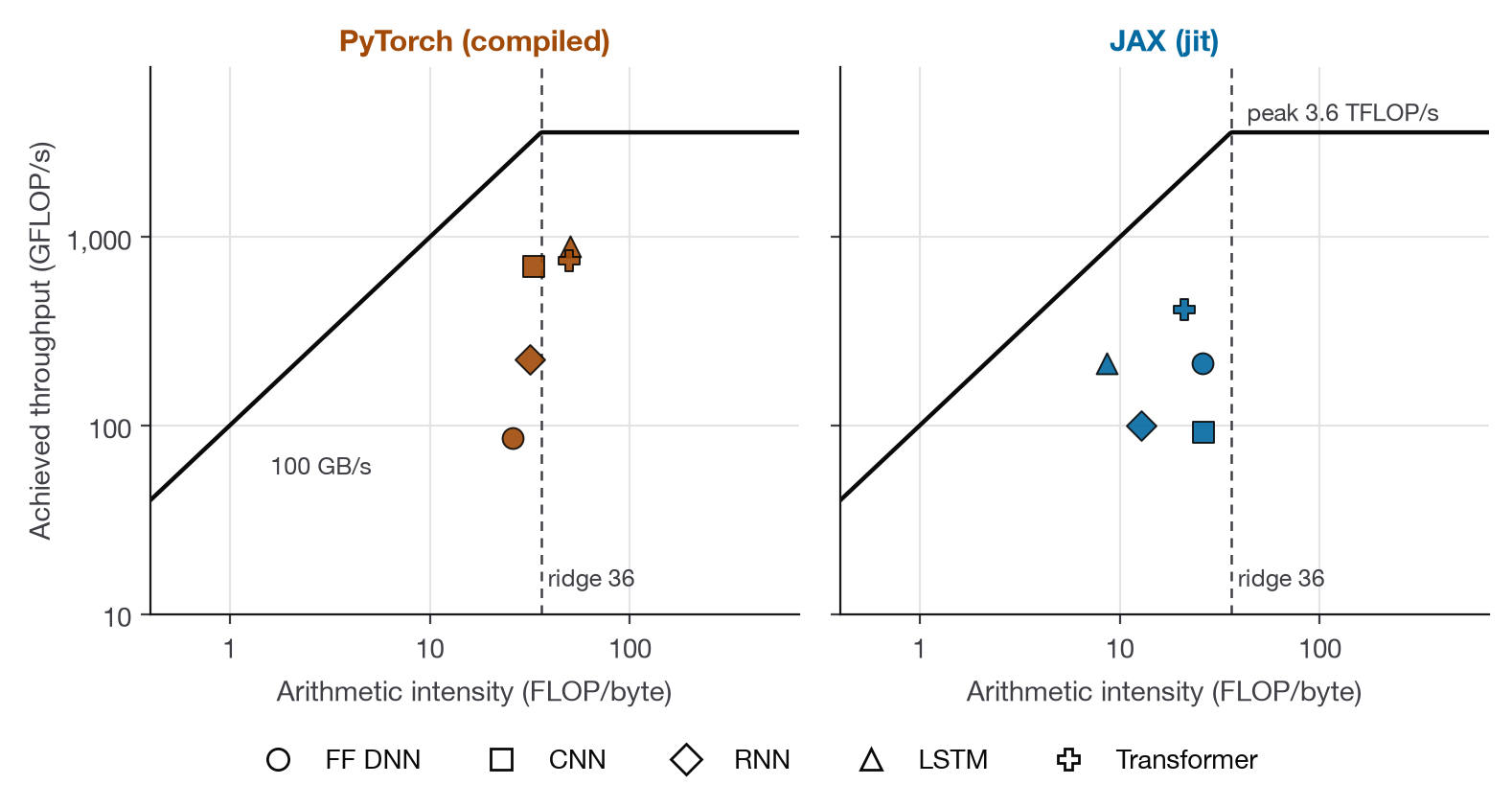
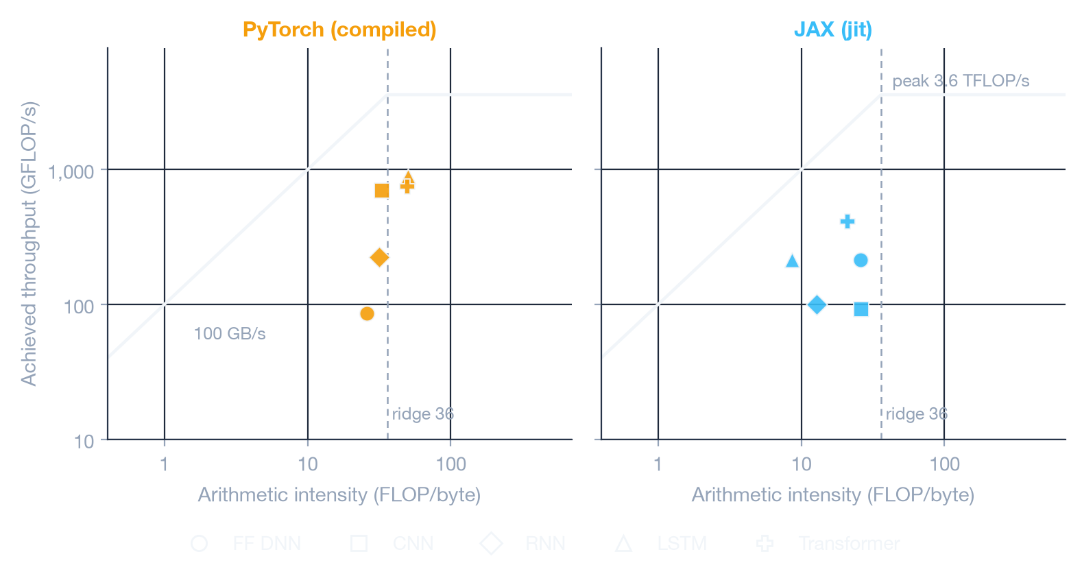
The roof is the same as on the CPU plot; the points moved. On PyTorch, the LSTM
( FLOP/byte) and Transformer ( FLOP/byte)
sit right of the 36 FLOP/byte ridge at 750–890 GFLOP/s, so they are compute-bound —
yet still only at 21–25% of the roof. Everything else is memory-bound. As in the CPU
post, JAX’s points sit further left because neural-cost’s JAX adapter counts traffic from
jaxpr primitives, so compare JAX on throughput rather than intensity.
Two things keep every point far below the ceiling at these sizes:
- Kernel launch overhead. Each dispatch to MPS carries a fixed scheduling cost, and a model this small issues many short kernels. Until the batch is large enough, that cost dominates.
- Small tensors. With , a single layer’s matrices are too small to keep the GPU’s parallel lanes busy. The smallest model, the FF DNN, is the one place the CPU still wins at batch=32 (see below).
Compiling barely moves these points; section 5 covers why.
2. Inference latency at batch=256
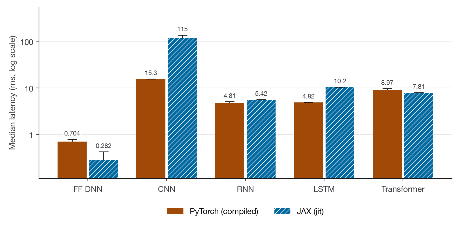
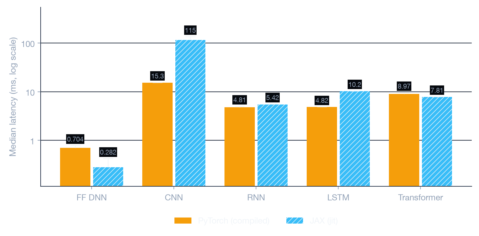
The benchmark sweeps batch sizes of 32 and 256. This section uses batch=256, where the GPU has the most work to chew on:
Full results table (batch=256)
| Architecture | Framework | Variant | Latency (ms) | GFLOP/s | Efficiency | Bottleneck |
|---|---|---|---|---|---|---|
| FF DNN | PyTorch | eager | 0.654 | 92.8 | 3.6% | memory |
| FF DNN | PyTorch | compiled | 0.704 | 86.3 | 3.3% | memory |
| FF DNN | JAX | eager | 0.295 | 205.3 | 7.9% | memory |
| FF DNN | JAX | jit | 0.282 | 214.8 | 8.3% | memory |
| CNN | PyTorch | eager | 15.397 | 694.7 | 20.9% | memory |
| CNN | PyTorch | compiled | 15.293 | 699.4 | 21.1% | memory |
| CNN | JAX | eager | 37.825 | 280.1 | 10.7% | memory |
| CNN | JAX | jit | 114.970 | 92.2 | 3.5% | memory |
| RNN | PyTorch | eager | 4.855 | 221.3 | 7.0% | memory |
| RNN | PyTorch | compiled | 4.809 | 223.4 | 7.1% | memory |
| RNN | JAX | eager | 6.586 | 81.9 | 6.4% | memory |
| RNN | JAX | jit | 5.424 | 99.5 | 7.8% | memory |
| LSTM | PyTorch | eager | 4.868 | 882.4 | 24.5% | compute |
| LSTM | PyTorch | compiled | 4.816 | 891.9 | 24.8% | compute |
| LSTM | JAX | eager | 18.211 | 119.1 | 13.8% | memory |
| LSTM | JAX | jit | 10.175 | 213.1 | 24.7% | memory |
| Transformer | PyTorch | eager | 7.273 | 927.1 | 25.8% | compute |
| Transformer | PyTorch | compiled | 8.970 | 751.7 | 20.9% | compute |
| Transformer | JAX | eager | 8.712 | 370.7 | 17.6% | memory |
| Transformer | JAX | jit | 7.806 | 413.8 | 19.6% | memory |
Bold marks the fastest run for each architecture.
LSTM and Transformer are the only architectures to break into compute-bound territory on PyTorch MPS at batch=256, reaching 21–26% roofline efficiency. That’s still far from saturation, but it confirms that parameter-heavy, attention and gate-heavy models benefit most from GPU parallelism.
3. Roofline efficiency heatmap
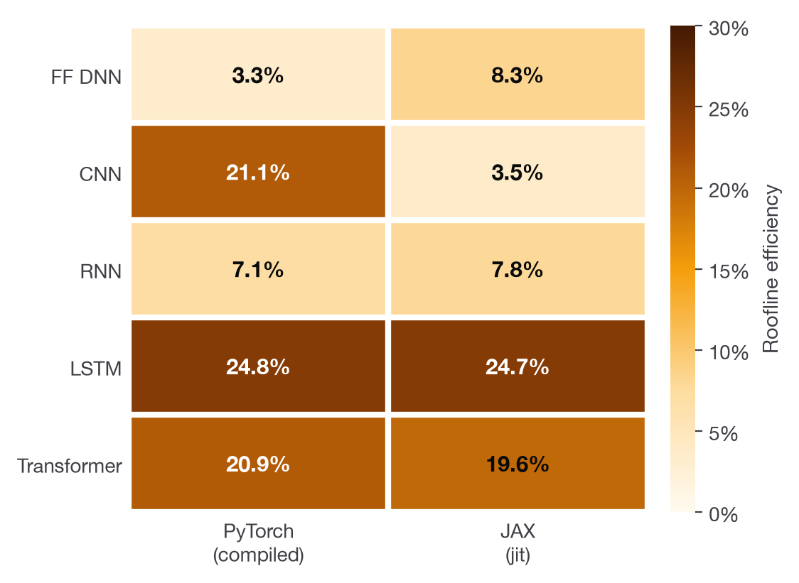
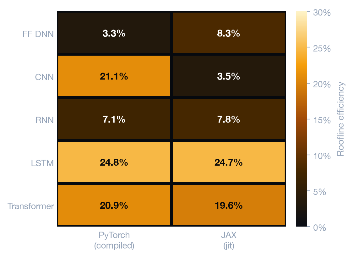
The CPU efficiency heatmap uses the same colour scale, so the two compare directly — with the caveat that the CPU numbers are at batch=32. GPU efficiency is higher in 6 of the 10 cells: PyTorch’s CNN, RNN, LSTM and Transformer climb from 2–8% to 7–25%. The FF DNN barely moves (3.3–8.3% on both devices), and JAX’s RNN drops from 10.0% to 7.8%.
The high-efficiency cells are instructive:
- LSTM (24.8% PyTorch, 24.7% JAX) — The gate-heavy LSTM with ~1.1M parameters produces enough arithmetic per weight byte to approach compute saturation on MPS.
- PyTorch Transformer (20.9% compiled, 25.8% eager) — Multi-head attention’s QKV
projection matrices fill the GPU’s parallel units well at batch=256. Eager mode is the
more efficient of the two here because
torch.compileregresses on this model.
4. Batch size scaling
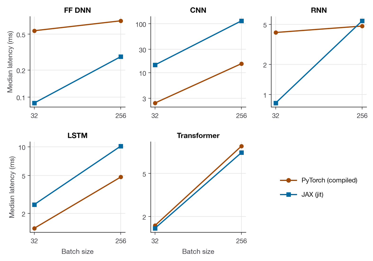
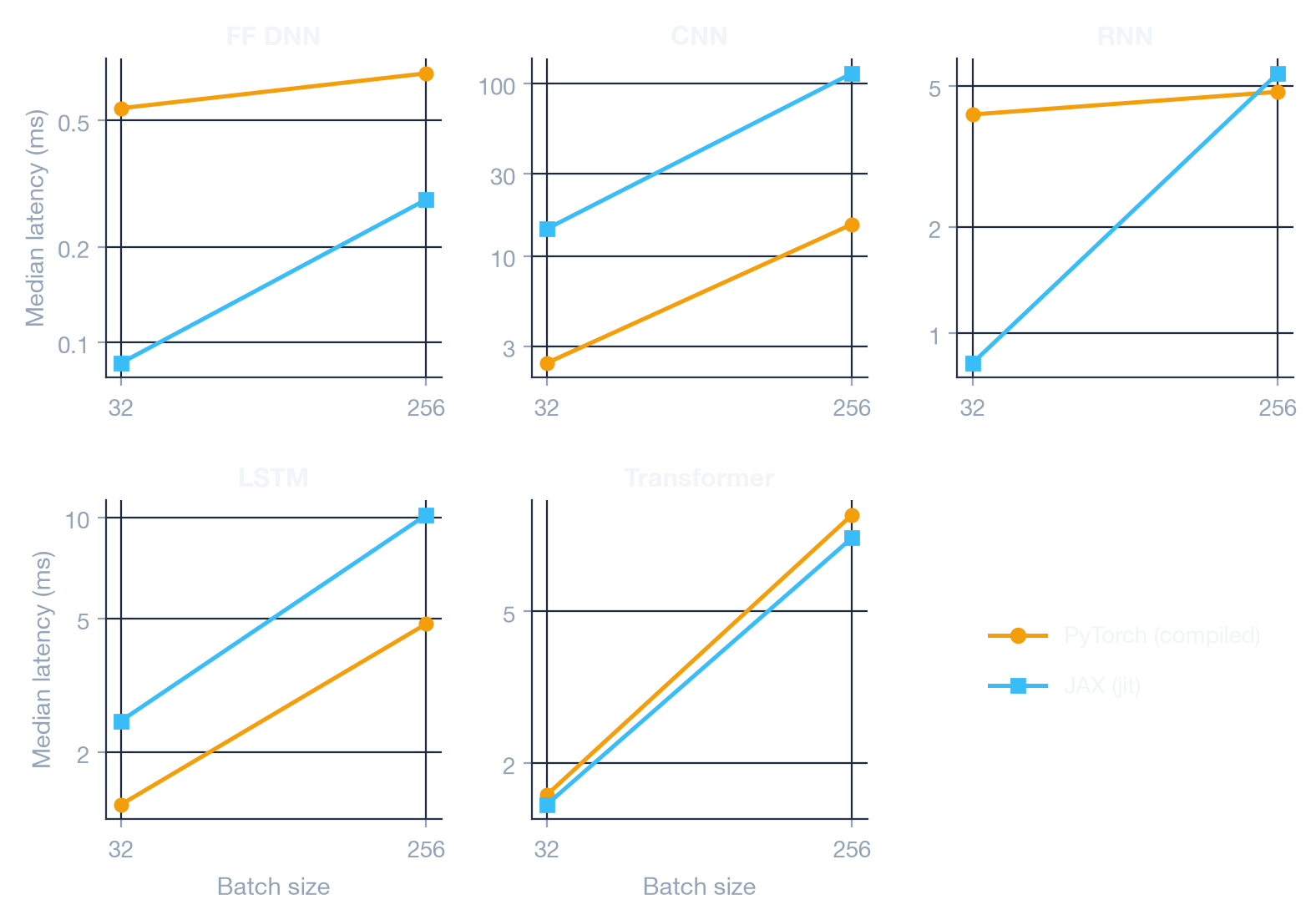
On CPU, latency grew roughly in proportion to batch size. On the GPU, going from batch=32 to 256 (8× the work) looks different:
- Latency grows sub-linearly almost everywhere — 1.2× to 6.6×. The parallel execution units finally have enough work to amortize launch costs, so throughput rises sharply. The exception is JAX’s CNN, which scales the full 8× (14.4 → 115 ms).
- Some models barely notice the extra work. PyTorch’s RNN goes from 4.15 to 4.81 ms and its FF DNN from 0.55 to 0.70 ms. At batch=32 they were almost entirely overhead.
This is the GPU utilization lever. Batch size is the single most important knob for GPU efficiency at these model sizes, more impactful than any compiler optimization.
5. Compilation and JIT speedups on GPU
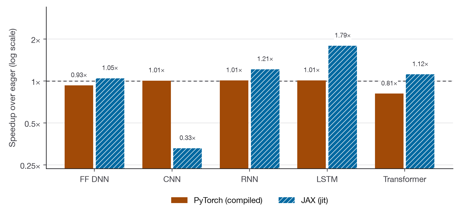
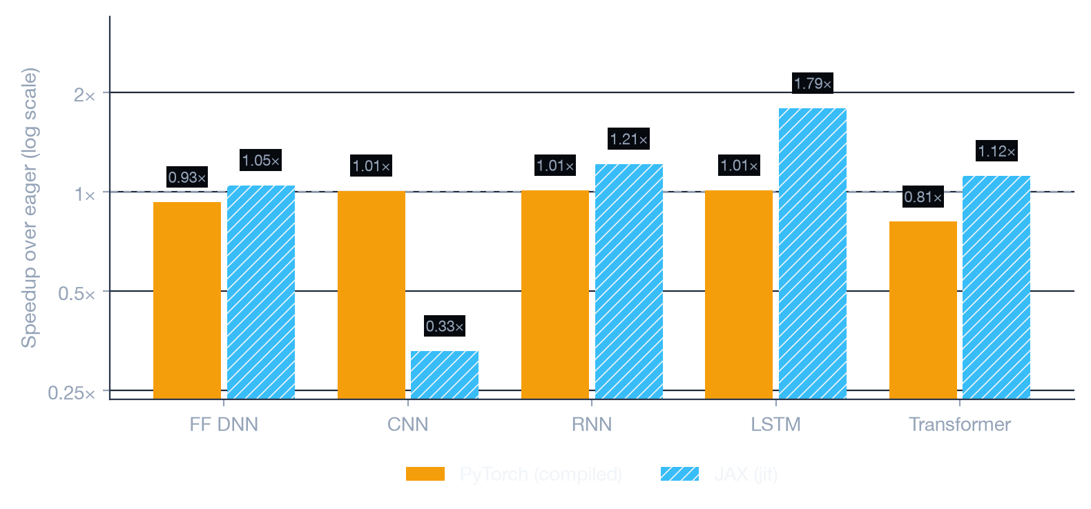
Speedup summary (batch=256)
| Architecture | PyTorch torch.compile | JAX jit |
|---|---|---|
| FF DNN | 0.93× (regression) | 1.05× |
| CNN | 1.01× | 0.33× (severe regression) |
| RNN | 1.01× | 1.21× |
| LSTM | 1.01× | 1.79× |
| Transformer | 0.81× (regression) | 1.12× |
The pattern mostly mirrors the CPU results,
where jax.jit gave 1.67–1.75× on the recurrent models and torch.compile was flat or slower:
jax.jit on LSTM delivers the largest GPU speedup (1.79×), reducing latency from
18.2 ms to 10.2 ms. XLA’s graph-level fusion eliminates intermediate tensor round-trips
through GPU memory — exactly the optimization that matters most on a memory-bandwidth-bound
device.
torch.compile regresses on FF DNN and Transformer, as it did on CPU. Torch’s
Inductor backend generates Metal compute shaders that can introduce extra synchronization
fences for small workloads, creating overhead that outweighs fusion gains.
JAX’s CNN regression (0.33×, latency 3× worse after JIT) is the most dramatic result in the dataset. Profiling indicates that XLA’s Metal convolution lowering inserts additional memory layout transposes when compiling static shapes for MPS, turning a well-tuned eager path into a slower compiled graph. The same JIT regression shows up on CPU (0.42×), so XLA’s convolution lowering looks like the common factor rather than MPS alone.
6. Achieved GPU throughput
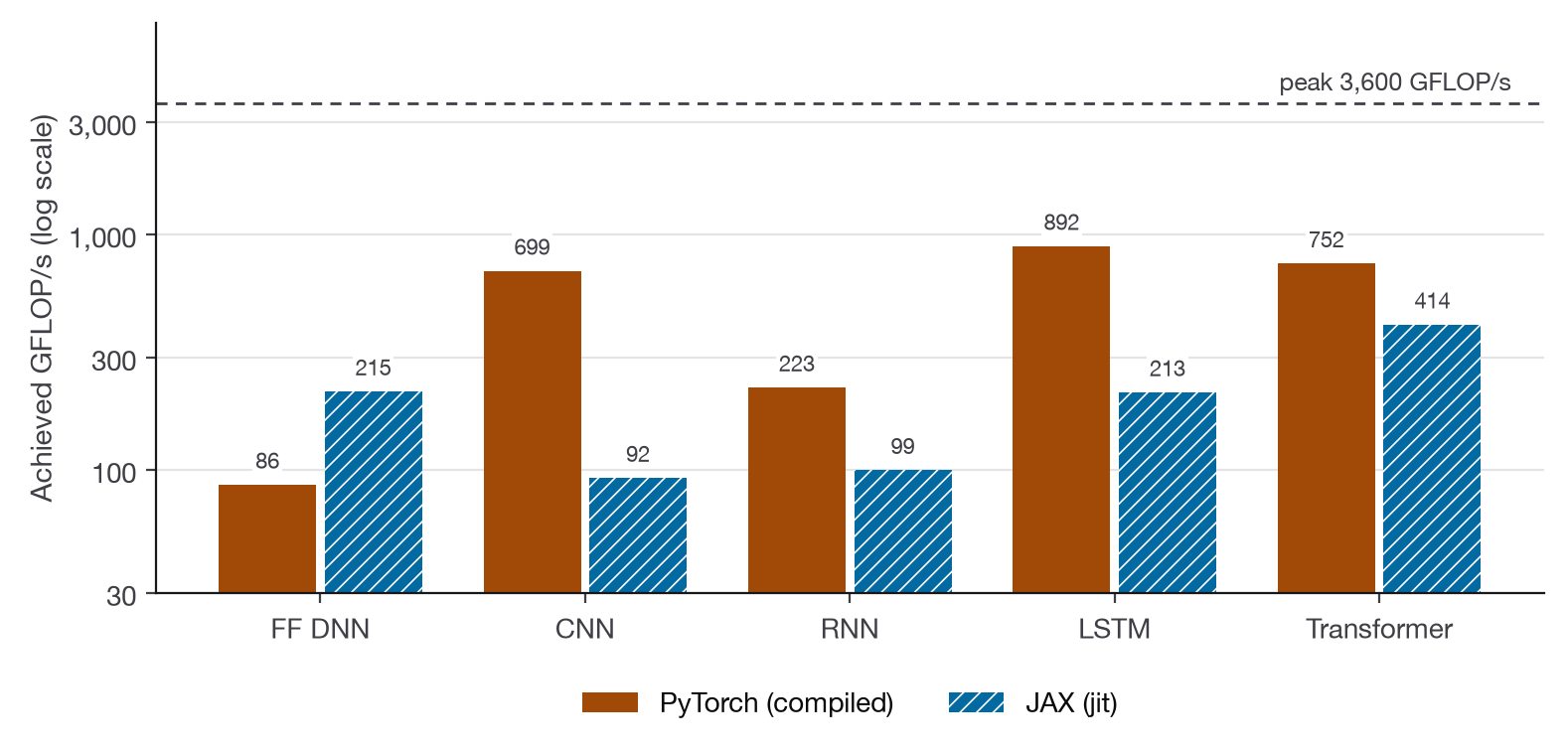
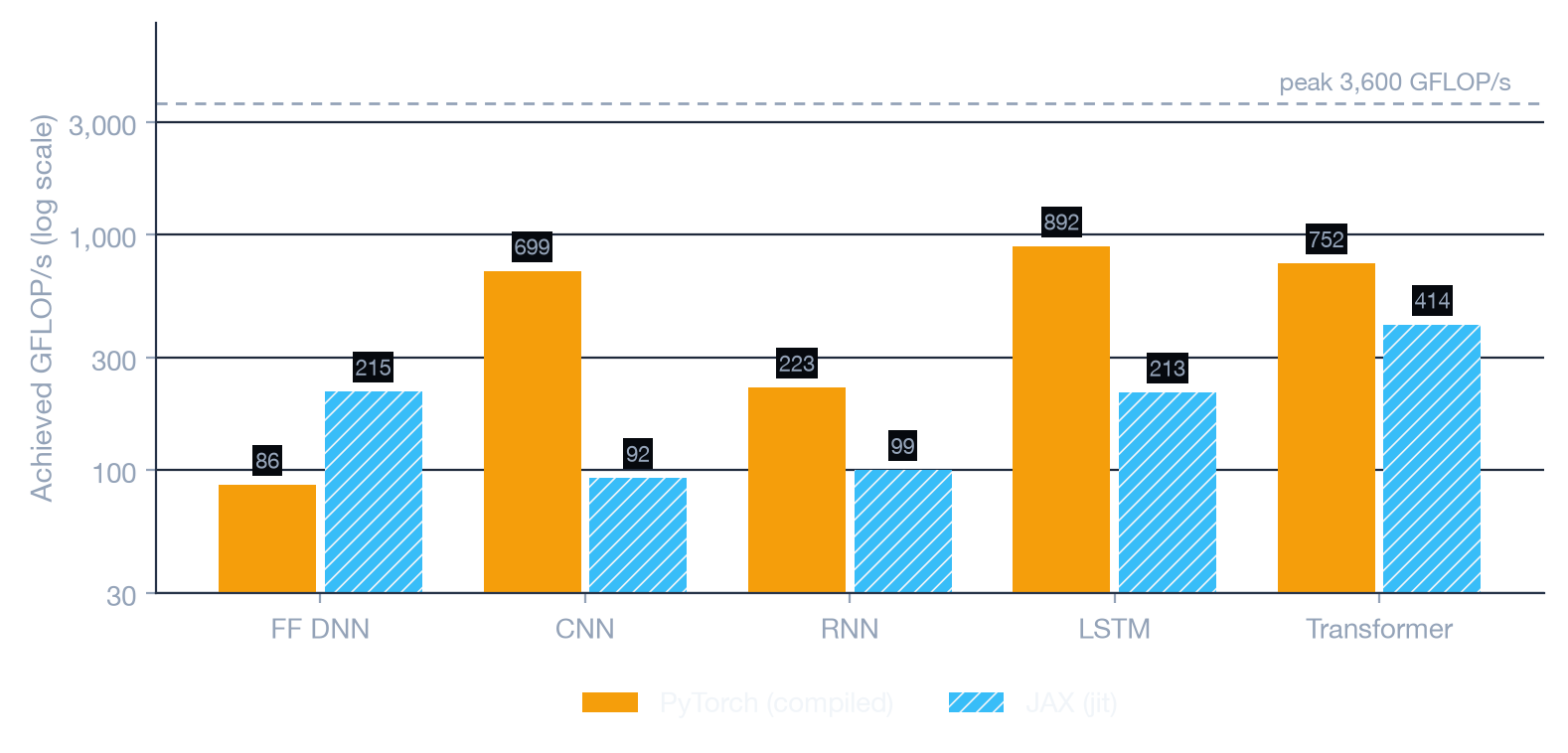
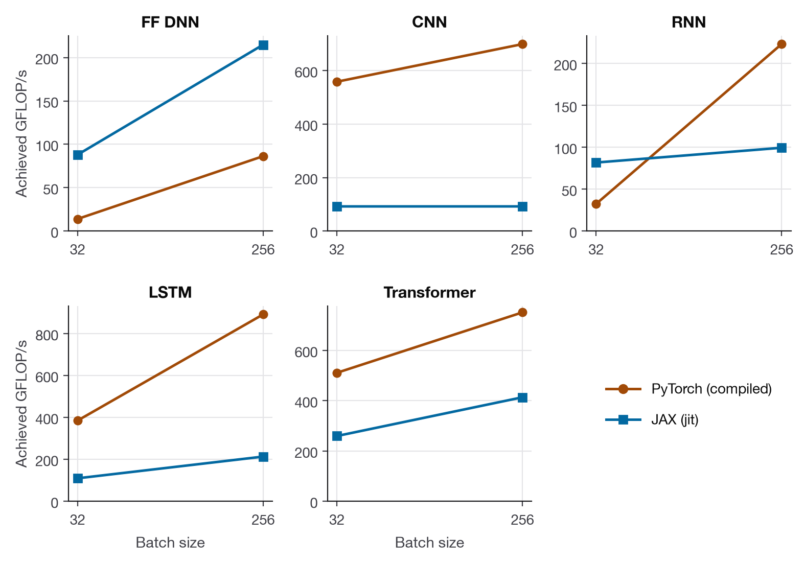
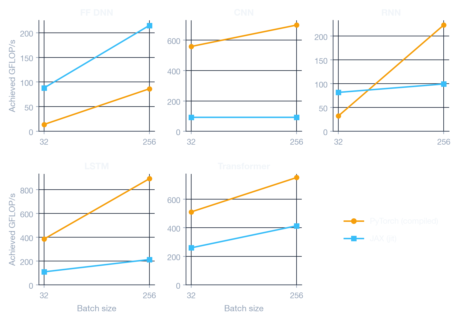
The throughput scaling curves show how GFLOP/s evolves as batch size grows from 32 to 256. The steepest climbs come from the models that were most starved at batch=32: PyTorch’s RNN (6.9×, 32 → 223 GFLOP/s) and FF DNN (6.2×), where launch overhead dominated. The LSTM and Transformer started much higher and rose a more modest 1.5–2.3×. JAX’s CNN doesn’t move at all (92 GFLOP/s at both sizes) — the JIT regression scales with the batch.
The key gap between PyTorch MPS eager and JAX eager throughput on the Transformer (927 vs. 371 GFLOP/s) reflects PyTorch’s more mature MPS kernel library. PyTorch’s Metal backend has received extensive optimization for attention and dense linear layers, while JAX’s MPS support remains experimental.
Architecture-by-architecture GPU winners (batch=256)
| Architecture | Fastest | Latency | Notes |
|---|---|---|---|
| FF DNN | JAX (jit) | 0.282 ms | 2.3× faster than PyTorch eager (0.654 ms) |
| CNN | PyTorch (compiled) | 15.293 ms | JAX JIT severely regresses on MPS Conv (115 ms) |
| RNN | PyTorch (compiled) | 4.809 ms | Minimal JIT gain; PyTorch MPS RNN kernel well-tuned |
| LSTM | PyTorch (compiled) | 4.816 ms | Compute-bound; 24.8% efficiency, the best of any compiled run |
| Transformer | PyTorch (eager) | 7.273 ms | JAX JIT is next (7.81 ms); torch.compile regresses to 8.97 ms |
PyTorch wins 4 of 5 architectures on GPU at batch=256 (vs. JAX winning 4 of 5 on CPU), driven by its more mature MPS kernel library for convolutions, RNNs, LSTMs and attention. JAX keeps the FF DNN, where XLA’s operation fusion outweighs PyTorch’s kernel quality. At batch=32 the split is closer: JAX wins the FF DNN, RNN and Transformer, PyTorch the CNN and LSTM.
GPU vs. CPU: when does the GPU actually win?
At batch=32 — the one batch size both benchmarks share — the GPU already beats the CPU’s best result on four of five architectures:
| Architecture | CPU, batch=32 (best) | GPU, batch=32 (best) | GPU, batch=256 (best) |
|---|---|---|---|
| FF DNN | 0.062 ms (PyTorch eager) | 0.076 ms (JAX eager) | 0.282 ms (JAX jit) |
| CNN | 5.012 ms (TF tf.function) | 2.393 ms (PyTorch compiled) | 15.293 ms (PyTorch compiled) |
| RNN | 0.893 ms (JAX jit) | 0.825 ms (JAX jit) | 4.809 ms (PyTorch compiled) |
| LSTM | 2.643 ms (JAX jit) | 1.395 ms (PyTorch compiled) | 4.816 ms (PyTorch compiled) |
| Transformer | 1.731 ms (JAX jit) | 1.555 ms (JAX jit) | 7.273 ms (PyTorch eager) |
The GPU is 2.1× faster on the CNN, 1.9× on the LSTM, and about 1.1× on the RNN and Transformer. Only the FF DNN — the smallest model — stays faster on CPU (0.062 vs. 0.076 ms): there isn’t enough work in it to pay for the dispatch.
The CPU sweep stopped at batch=128, so batch=256 latencies have no direct CPU counterpart. Throughput is the fairer comparison there: PyTorch’s LSTM on the GPU processes about 53,000 samples/s at batch=256, against about 14,300 samples/s for the CPU’s best LSTM run at batch=128 (JAX jit) — roughly 3.7× more. In GFLOP/s it’s 892 against the CPU’s best of 185 (TensorFlow at batch=128).
Conclusions
1. Batch size is the primary GPU utilization lever
The roofline analysis makes the mechanism explicit: increasing batch size raises arithmetic intensity (FLOPs per memory byte), pushing workloads toward the compute-bound regime. Going from batch=32 to 256 raised PyTorch’s throughput 1.25–6.9× while latency grew far less than the 8× increase in work. We didn’t measure beyond 256, so whether the LSTM and Transformer get much closer to the compute roof at 512 is still an open question.
2. JIT compilation helps selectively — about as much as on CPU
jax.jit gives 1.05–1.79× on GPU (1.06–1.75× on CPU) and regresses on the CNN on both
(0.33× and 0.42×). torch.compile is flat or slower on both. Compilation enables kernel
fusion that eliminates intermediate memory round-trips, but only when the backend’s
lowering is mature. The large CPU wins came from tf.function bypassing Python dispatch,
and TensorFlow wasn’t part of the GPU run.
3. PyTorch’s MPS kernel library is more mature than JAX’s
JAX won 4 of 5 CPU categories but only 1 of 5 GPU categories at batch=256 (3 of 5 at batch=32). The reversal reflects PyTorch’s multi-year investment in production MPS kernels for convolution, recurrent and attention workloads. As JAX’s MPS backend matures, this gap should close.
4. Small models need only a modest batch for the GPU to pay off
For model architectures at , the GPU already beats the CPU at batch=32 on everything except the FF DNN. Batch=1 wasn’t measured on the GPU, so for single-request inference the CPU numbers are the only data here — and the FF DNN result suggests the smallest models are better left on the CPU. If your deployment can batch even 32 requests together, the GPU is worth measuring.
What’s next for neural-cost
The v0.2.0 GPU path opens up several directions on the roadmap:
- NVIDIA CUDA support — CUDA event timing and
nvidia-smipower sampling to extend roofline analysis to datacenter GPUs. - Activation checkpointing model — re-materialization changes the FLOPs/memory tradeoff significantly; the static estimator will gain a checkpoint-aware mode.
- Distributed communication cost — all-reduce and pipeline communication costs don’t appear in per-device FLOPs counts; collective bandwidth modeling is on the list.
- Per-op kernel traces on JAX — current JAX and TF adapters use allocator-level telemetry; per-kernel XLA HLO traces would close the gap with PyTorch’s profiler.
Code and reproducibility
All benchmark scripts, raw JSON telemetry, and figure generators are open-source:
- neural-cost v0.2.0:
davidgraymi/neural-cost· taggedv0.2.0 - GPU data collector:
benchmarks/collect_gpu_data.py - Report generator:
benchmarks/generate_gpu_report.py - Raw telemetry:
benchmarks/results/benchmark_gpu_data.json
See also the companion posts:
- neural-cost: Roofline Analysis Across PyTorch, JAX, and TensorFlow — library internals and API
- PyTorch vs. JAX vs. TensorFlow: A Roofline Benchmark Across 5 Architectures — CPU baseline results
Updated October 19, 2026: the CPU-vs-GPU table previously showed batch=256 GPU latencies in its batch=32 column, which led to the wrong conclusion that the GPU loses at batch=32. The table, the conclusions that depended on it, and several figures quoted in the text have been corrected, and the charts were regenerated from the same raw data.